Appendix 6 The Concept of Experimental Error and its Statistical Basis
To understand what is meant by the term "error" in the
context of experimental measurement, consider the first
experiment you did in C10J practicals - the determination of the
acetic acid content of a sample of vinegar. Let's say you
obtained a value of 4.79%. It is quite reasonable to ask of you
(and your instructor who designed the experiment) how sure you
both are that this result is the true value. How likely is it
that you would obtained this same exact value again, if you
repeated the experiment on a similar sample of vinegar, using
very similar volume measuring devices, and using the same
technique?
The answer of course is that it is very likely that you
would not obtain this exact same value, even if
you repeated it several times. A sceptical fellow student
(especially one who is doing some philosophy) might well ask what
good is your measurement if it is not likely to give the same
result consistently. The truth is that if you repeated the
measurement several times, you are likely to obtain values like
those listed below:
| 4.89 |
4.95 |
4.76 |
4.69 |
4.85 |
| 4.63 |
4.78 |
4.75 |
4.74 |
4.86 |
| 4.79 |
4.80 |
4.66 |
4.80 |
4.75 |
(These values were actually obtained by members of a former C10J
class). One can see that the numbers are not just totally random
- they range in value from 4.63 to 4.95, and are really not so
very different at all from the single value you obtained. In fact
if we were to collect all 50 values obtained by your classmates
any one day, and plot a frequency distribution of the values, in
groups, we are likely to obtain a plot similar to that shown
below.
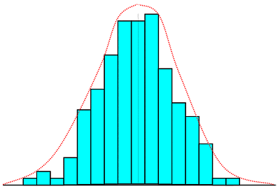
The bar graph shows a typical distribution of say 50-odd
data points, while the dashed line shows the distribution likely with large number of data points
plotted in very narrow-width groups.
(A frequency distribution is the plot of the number of times a
value occurs within a group, say 4.75 - 4.85, plotted against the
group value). As you can see, this results in a fairly
symmetrical pattern of distribution of values about a central
value. The distribution is one which is fairly well known to
statisticians. It is known as a Gaussian or
normal distribution, but what is more important for us,
is that it has properties which tell us quite a bit about the
likelihood of obtaining certain values for our
measurement, and that is exactly what we want to know.
When the results of repeated similar experiments follow a normal
distribution we know that the most probable value of the
quantity we are measuring is the mean (or average)
value. We find also that 95% of the values obtained by repeating
the experiment will fall between (the mean - 2σ) and (the mean +
2σ) where s is a measure of the broadness of the distribution.
Also, 68% of the values can be expected to fall between (the mean
- σ) and (the mean + σ).
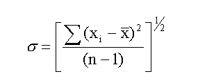
The quantity σ is a measure of dispersion used by statisticians,
and it is knows officially as the standard deviation or
the standard error of the set of data. The formula for
calculating σ is
The denominator, (n-1) is used instead of n when the sample is
small (< 30). xbar is the mean value and (xi - xbar) is the deviation
of each data point from the mean.
Applying this formula to the 15 data points listed
earlier gives a standard deviation of 0.085, with the mean value
being 4.78. The meaning of this result can be stated thus:
"95% of the values obtained by students in the lab group from
which the sample is drawn, are likely to fall between 4.61 and
4.95, i.e. (4.78 ± 0.17) and 68% are likely to fall between 4.69
and 4.87, i.e. (4.78 ± 0.09)."
We can view this another way. For any single determination of x,
there is a 95% probability that the mean will fall between (x -
2s) and (x + 2s) and 68% that it will fall between (x - s) and (x
+ s). When it is viewed this way , it is obvious that s is a
measure of the error (or uncertainty) associated with the
experimental determination of x. But what should we write as the
error, ±s or ±2s? We can write either, as long as we make it
clear which one is being written. The latter (±2s) is quite a
conservative estimate and even the former (±s) represents better
than 50% certainty that the mean falls within the range
specified. (The value which represents 50% certainty is in fact
known as the probable error and it turns out to be
±0.67s). For reasons which we will see later, it is it is the
most probable error that is usually written as the error in
measurements. However it does not make a great deal of difference
if we regard the error as ±s.
So, if we had known the value of σ, we could
have written the result of our single measurement as:
acid content = (4.79 ±0.09)%
The result could then have been interpreted (to your
philosophical fellow student, for example), to mean that if you
had repeated the experiment several times using the same
equipment and technique, the average of these repeated
determinations is very likely to fall within the range 4.70 to
4.88.
One begins to really appreciate the importance of this
statement of error, when one is asked to make a judgement on the
value obtained for the acid content of vinegar. Suppose, for
example, that the label on the product, as it is sold on the
market, claims that the acid content is 6.5%, could we use your
single result as the basis for saying that the producer has
labelled the this product wrongly? The answer would of course be
yes. For if we know the value of s to be 0.085, we are
quite confident (95%) that the acid content is somewhere within
the range 4.61 to 4.95.
We might wish in fact to improve our confidence in the
value, by doing the determination once or twice again, using the
mean of these determinations instead of the single value, as our
experimental result. We might also wish to check that our
reagents were really as pure as we assumed, and that our standard
NaOH was indeed the molarity stated, before we made any public
accusations. It should be quite clear however that we can make
judgements based on our results, provided we know what
uncertainty or error we can reasonably associate with these
results. Conversely it would be fair to say that your result has
no real use or meaning if you have no idea of the uncertainty
associated with that result.
Types of Error, Accuracy and Precision
It should be evident from our discussion so far that
experimental errors exist and are present (to some extent) in all
experimental measurement. Our task as experimental scientists
must therefore be to design experiments to produce the best
results we can, in spite of such errors, and to assess the
uncertainty which these unavoidable errors cause in our
measurement.
It is useful to distinguish between two types of
experimental error - systematic (or bias) error, and random
error, though the distinction can appear to be somewhat
artificial in some cases.
Systematic error is experimental error whose
numerical value tends to remain constant, or follow a consistent
pattern over a number of experimental runs. In the determination
of the acid content of vinegar, systematic error would have been
introduced if the standard sodium hydroxide was of a lower
molarity than it is said to be. Suppose its molarity was
determined from the mass of NaOH pellets made up to say 500 cm3.
This, apart from being bad practice, would almost certainly
introduce systematic error into the determination because NaOH
pellets absorb water from the atmosphere very rapidly, when they
are being weighed.
The mass of water absorbed would have been interpreted as
mass of NaOH and so the true molarity would have been
less than that calculated. The molarity of acid
determined by titration against this base would turn out to be
systematically greater than the true value.
We can generalize a bit and say that systematic error
arises from incorrect procedure, incorrect use of
instruments, or failure of some value to be what it is assumed to
be.
Random error, on the other hand, is experimental
error whose numerical value and sign are likely to change from
one measurement to the next. The average value for random error
is zero, and it is the random error in measurements which cause
the frequency distribution of repeated experimental results to
follow the normal or Gaussian distribution mentioned earlier.
The error which arises because one does not have ones
eyes exactly level with the bottom of the meniscus, when reading
a burette, is usually random error. Sometimes the eyes will be
above the level and the reading will be greater than the true
value, while some times the eyes will be below the level and the
reading will be less than the true value (usually by small
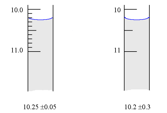
amounts). Many of you already have a "rule of thumb" for
estimating random error in readings such as that of a burette -
the error being approximately ± a half of the smallest division.
This is a good estimate in some cases, but not so good in others,
as is illustrated below:
These two types of errors usually have very different
effects on the results of an experiment. To illustrate this, we
took 30 results of students doing the determination of the acid
content of vinegar on a different lab day from those already
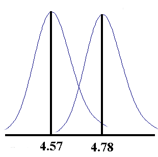
given. These results had a mean of 4.57 and a standard deviation
of 0.068, (compared to 4.78 and 0.066). The distribution from
which these samples are drawn can be represented by the two
curves shown below.
Systematic errors account for the shift in the mean from one day
to the next, while random errors account for the spread of the
values about the mean each day. The random error can be seen to
be associated more with the technique and instrumentation used,
from the fact that it is about the same each day the experiment
is done.
What do you think is the cause of the systematic difference
between the results? We say that systematic error affects the accuracy of the result -
i.e. its closeness to the 'true value, while ramdom error affects
the precision or repeatability of the results. The 'true' value
is simply the best available experimental value, in our case. For
universal constants such as R, the gas constant, and h, Plank's
constant, the true or accepted value is the mean of the values
obtained by the best experiments done by different workers.
Coping with Errors in Measurement
Systematic errors can be identified and their effect
reduced, by putting some thought into the design of the
experiment, to ensure in particular that experimental conditions
are controlled, the equipment is appropriately calibrated and
that any assumptions which are inherent in the technique, are
adequately met in the conditions selected.
In the experiment to determine the acid content of
vinegar, good practice would require that each batch of
"standard" NaOH is standardized against a good reproducible
standard such as pure potassium hydrogen phthalate, and that an
indicator which changes near the equivalence point (pH » 8.0) is
used. This ensures that the assumption that the acid and base are
present in equivalent number of moles, is valid in our
experiment. These and other features of the design which are
aimed specifically at reducing systematic error are usually not
recognized by those who follow the instructions in recipe-like
fashion. But how does one decide which of the two lab days had
the more accurate result?
If all else fails, a good check on the accuracy of the
result would be to have the determination done independently,
elsewhere - perhaps by a completely different method in a
non-University lab. Agreement between two such independent
determinations is very strong support for any claim of accuracy.
When it is not possible to have such independent checks done,
"internal" monitoring of accuracy can be achieved by determining
an accurately known standard of acetic acid with each new batch
of reagents used, and by determining this standard as part of the
routine on each lab day.
The strategy for dealing with random error is some what
different, for it relies mainly on repeating the same experiment
a number of times. The rationale for this approach is simply the
fact that the average of a number of observations is more precise
than a single observation. In the acetic acid determination the
mean of 33 values, 4.78, is more precise than the single value
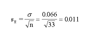
obtained by any individual. The standard error in the mean is
given by the statistical considerations as
So whereas the single value has a standard error of
0.066, the mean has a standard error of 0.011.
Since the value of 1/√n decreases very rapidly for
increasing n, when n is small, it is good practice to repeat the
determination a couple of times, if you want to be a bit more
confident about your results. That is why it was recommended
earlier that you repeat the determination of acetic acid in
vinegar at least once or twice before making accusations against
the manufacturer.
Medical laboratories usually do their determinations in
duplicate or triplicate for this reason, and many of the run
"internal" standards with each batch of samples, as a means of
checking on changes in the accuracy of the procedure from week to
week.
Of course it follows that more precisely calibrated
instruments will help to improve precision. A thermometer which
has its smallest division as 1°C is likely to have reading errors
of about ±0.5°C, (i.e. half of the smallest division), while one
with ten divisions per 1°C can be read to about ±0.05°C.
Lastly it should be pointed out that you do not need to
have the most accurate and most precise instruments available to
do every measurement. For example it is usually sufficient to
determine the melting point of a substance to ± a tenth of a
degree Celcius to ascertain its purity for most practical
purposes in Organic labs. But a thermometer is required which is
fairly accurate, because it is the absolute value of
the temperature on which the assessment of purity is based.
On the other hand the measurement of the temperature
change which accompanies the dissolution of 1 g of potassium
nitrate in 100 cm3 of water, (about 0.50°C), requires a more
precise measurement, perhaps to ± a hundredth of a
degree Celcius. The absolute accuracy of the thermometer is not
all that critical because the assessment here is based on a
temperature difference.
When you put 2 kg of water into the jacket of a bomb
calorimeter, you need to know this with a precision of only ± 1 g
to have a 0.05% precision, but when you weigh out 2 g of
potassium phthalate to make up standard solutions you need to
know the mass to ± 1 mg in order to have the same precision.
Estimating Error in a Single Determination
The random error which one should ascribe to an
experimental result has been shown to be ± s. So far we have seen
this standard error determined only from statistical analysis of
a number of repeated determinations of the experimental result.
The question of what to do when you have made only one or two
determinations of the experimental quantity, is still unanswered.
It is an important question because in most of our experiments we
have time to determine the final value only once, even though we
may do duplicate determinations of some primary quantities in the
procedure.
We do already have some idea of the error associated with
the measurement of individual primary quantities like volume,
time and mass, (± ½ the smallest division), and it seems
reasonable to assume that if we combine these errors, using the
methods of statistics, we should end up with a good estimate of
the error in the final result. In fact, most of you already make
some estimate of error in your final result by taking the sum of
the percentage errors in the various primary measurements. This
is not quite correct from a statistical point of view. It is in
fact the square root of the sum of the squares of the errors, or
percentage (relative) errors that really represents the combine
error.
The following rules can be used to give a reasonable
estimate of the combined error in your final result.
(a) For sums and differences the actual error in the result is
the square root of the sum of the squares of the actual errors in
the contributing terms:
If,
A(±a) . B(±b) = C(±c)
where a is the actual error in A, etc. then
c = (a2 + b2)½
EXAMPLE A titre volume which is usually obtained by
taking the difference in burette readings before and after
titration, will have a combined error of each reading (± 0.05
cm3) given by:
Final reading 18.30 ± 0.05 cm3
Initial reading 5.05 ± 0.05 cm3
Titre volume 13.25 ± ?
c = [(0.05)2 + (0.05)2]½ = 0.07 cm3
Titre volume = 13.25 ± 0.07 cm3
(b) For products and quotients the relative (or
percentage) error in the results is the square root of
the sum of the squares of the relative (or percentage)
errors in the contributing terms.
If,
A(±a) x B(±b) = D(±d)
then,
EXAMPLE Consider the case of the molarity of acetic
acid determined from titration against standard NaOH.
Macid = (MNaOH. VNaOH) / Vacid
If we represent the error in each quantity as D(quantity), we
have
Assuming that the error in the 10 cm3 pipette, used to
take the sample of acid for titration, is about ± 0.05 cm3; and
assuming negligible error in the molarity of NaOH, we have
So the relative error in the acid molarity is 0.0073 or
0.7% (using some actual data taken from a C10 student).
(c) To calculate the error in the final result, arrange the
equation (used to get the result) in its simplest form, and
combine errors using the rules given above. You may neglect any
error (or a relative error) which is less than a tenth of the
largest error (or relative error).
EXAMPLE
In the case of the acetic acid determination, we already have
established in the above example that ~ 0.7% error exists in the
molarity of the diluted acid due to uncertainty of the volumes
used in titration. But there is also an uncertainty due to the
fact that you took an aliquot of 10.00 ± 0.05 cm3 of the acid and
diluted that up to 100.0 ± 0.2 cm3. Both uncertainties contribute
to the error in the dilution factor resulting in an uncertainty
of about 0.053 in 10.00, the error in the volume of the diluted
acid being almost negligible.
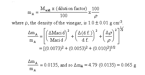
The final result which is the mass of acetic acid in 100 g of
vinegar is given by mA, where
We have estimated the error in our single value, 4.79,
and found it to be approximately ± 0.065. This is really quite a
good estimate considering that the value determined from the
statistical spread of 33 repeated values was ± 0.066. This
agreement between the two is better than what one would normally
expect, but it does make the point that good estimates of error
can be made for an experimental result by considering the error
involved in the individual primary measurement.
It is this "art" which we hope you will develop.
Accordingly we expect you to do an error analysis in every
experiment you do in the Physical Chemistry Lab, and will treat
it as an integral part of your report on lab-work for purposes of
assessment.
Significant Figures
Every measurement should be recorded to as many figures
as are significant, and no more. Wherever possible the
uncertainty of the measurement should be recorded, but if it is
not known, it is assumed to be uncertain by ± 1 in the last
digit.
Those zeros in a number which locate the decimal point
are not significant; 0.00314 and 80200 each have three
significant figures. The exponential (scientific) notation,
8.0800 x 10⁴ should be used.
The logarithm of a number should have as many
significant figures in the mantissa as there are significant
figures in the number.
Example antilog 0.032 = 1.08. The result shows three
significant figures in the mantissa.
Note that in the case of logarithms, the zero of the mantissa
is counted.
The number of significant figures of a computed
result is limited by the term with the largest uncertainty. In
addition and subtraction, the number of significant figures in
the result depends on the term with the largest absolute
uncertainty.
Example: 1.9546 g + 2.03 g = 3.98 g. The result is
expressed only to the nearest 0.01 g because 2.03 is only
expressed to the nearest 0.01 g.
Example: 68.7 cm - 68.42 cm = 0.3 cm. This result is
expressed only to the nearest 0.1 cm because 68.7 cm is only
expressed to the nearest 0.1 cm.
In multiplication and division, the number
of significant figures in the result depends on the term with the
largest relative uncertainty. The relative uncertainty
of a quantity is the absolute uncertainty divided by the value of
the quantity.
Example: 0.26 cm x 21.902 cm2 = 5.7 cm3. The result is
expressed to two significant figures because the relative
uncertainty in 5.7 cm, 0.1/5.7 or 1.8%, is about the same as that
in 0.26 cm, 0.01/0.26 or 3.8%. In multiplication and division the
number of significant figures in the result is usually equal to
that of the term with the least number of significant figures. In
some cases, however, the result may have a greater number of
significant figures than that of the term containing the least
number of significant figures.
Example: 1049 g/94 g mol-1 = 11.2 mol and not 11 mol.
The result is expressed to three significant figures rather than
to two because the relative uncertainty of 11.2 mol, 0.1/11.2 or
0.9%, is about the same as that for 94 g mol-1, 1/94 or 1.1%,
while that of 11 mol, 1/11 or 9.1%, is much larger.
In performing extended calculations, one should carry along
one more than the allowed number of significant figures. When the
answer is obtained, it can be rounded off to the correct number
of significant figures.
In rounding off a number the following rules should be
observed:
When a number smaller than 5 is dropped, the last remaining digit
is left unchanged: when a number larger than 5 is dropped, the
last remaining digit is increased by one digit: When the number
to be dropped is a 5 followed by a 0, the last remaining digit is
rounded off to the nearest even digit.
Example: The following numbers are rounded off to 3
figures: 1.7348 becomes 1.73; 1.735 becomes 1.74.
 Return to Chemistry, UWI-Mona,
Home Page
Copyright © 1995-2009 by The Department
of Chemistry UWI, Jamaica, all rights reserved.
Created and maintained by Prof. Robert J.
Lancashire,
The Department of Chemistry, University of the West Indies,
Mona Campus, Kingston 7, Jamaica.
Created Mar 1995. Links checked and/or last
modified 19th October 2009.
URL
http://wwwchem.uwimona.edu.jm/lab_manuals/c10appendix6.html




 Return to Chemistry, UWI-Mona,
Home Page